5.2 Summary metrics

In this vignette, we aim to evaluate the contribution of individual species and sites to each bioregion using the function site_species_metrics(). We also show how various metrics at the bioregion level can be computed, in particular with the function bioregion_metrics().

1. Data

We use the vegetation dataset included in the bioregion.

data("vegedf")
data("vegemat")

# Calculation of (dis)similarity matrices
vegedissim <- dissimilarity(vegemat, metric = c("Simpson"))
vegesim <- dissimilarity_to_similarity(vegedissim)

2. Bioregionalization

We use the same three bioregionalization algorithms as in the visualization vignette, i.e., non-hierarchical, hierarchical, and network bioregionalizations. In addition, we include a network bioregionalization algorithm based on a bipartite network, which assigns a bioregion (or cluster) to both sites and species. We chose three bioregions for the non-hierarchical and hierarchical bioregionalizations.

# Non hierarchical bioregionalization
vege_nhclu <- nhclu_kmeans(vegedissim, 
                           n_clust = 3, 
                           index = "Simpson",
                           seed = 1)
vege_nhclu$cluster_info

##     partition_name n_clust
## K_3            K_3       3

# Hierarchical bioregionalization
set.seed(1)
vege_hclu <- hclu_hierarclust(dissimilarity = vegedissim,
                              index = "Simpson",
                              method = "average", 
                              n_clust = 3,
                              optimal_tree_method = "best",
                              verbose = FALSE)
vege_hclu$cluster_info

##   partition_name n_clust requested_n_clust output_cut_height
## 1            K_3       3                 3            0.5625

# Network bioregionalization
set.seed(1)
vege_netclu <- netclu_walktrap(vegesim,
                               index = "Simpson")
vege_netclu$cluster_info

##     partition_name n_clust
## K_3            K_3       3

# Bipartite network bioregionalization
install_binaries(verbose = FALSE)
vege_netclubip <- netclu_infomap(vegedf,
                                 seed = 1, 
                                 bipartite = TRUE)
vege_netclubip$cluster_info

##     partition_name n_clust
## K_8            K_8       8

3. Species-to-bioregion & site-to-bioregion metrics

Several metrics evaluating the contribution of a species or a site to each bioregion can be computed and further aggregated to assess the relationship between a species or a site and the bioregionalization.

3.1 Species-to-bioregion metrics

Species-to-bioregion metrics are based on a bioregionalization containing \(K\) bioregions (vege_nhclu computed above for example) and its associated site–species co-occurrence matrix vegemat to compute three core terms, from which occurrence-based indices are derived.

\(n_{sb}\) is the number of sites belonging to bioregion \(b\) in which species \(s\) is present.
\(n_s\) is the total number of sites in which species \(s\) is present.
\(n_b\) is the total number of sites belonging to bioregion \(b\).

nsb <- site_species_metrics(bioregionalization = vege_nhclu,
                            bioregion_indices = "CoreTerms",
                            bioregionalization_indices = NULL,
                            data_type = "occurrence",
                            node_type = "site",
                            comat = vegemat,
                            similarity = NULL,
                            index = NULL,
                            verbose = FALSE)

nsb$species_bioregions[1:10,]

##    Species Bioregion n_sb n_s n_b
## 1    10001         1   27 254 358
## 2    10001         2   97 254 150
## 3    10001         3  130 254 207
## 4    10002         1    5  19 358
## 5    10002         2    1  19 150
## 6    10002         3   13  19 207
## 7    10003         1   82  86 358
## 8    10003         2    0  86 150
## 9    10003         3    4  86 207
## 10   10004         1  205 438 358

These core terms and associated indices are computed when data_type = "occurrence" (or data_type = "both") and node_type = "site" (or node_type = "both"). node_type = "site" means that a bioregion is assigned to each site in vege_nhclu.

Several metrics can be derived from these core terms.

Specificity (occurrence)

The specificity \(A_{sb}\) of species \(s\) for bioregion \(b\) (De Cáceres & Legendre, 2009) is defined as

\[A_{sb} = \frac{n_{sb}}{n_s}\]

and measures the fraction of occurrences of species \(s\) that belong to bioregion \(b\). It therefore reflects the uniqueness of a species to a particular bioregion.

NSpecificity (occurrence)

A normalized version that accounts for the size of each bioregion is also available, as defined in (De Cáceres & Legendre, 2009):

\[\bar{A}_{sb} = \frac{n_{sb}/n_b}{\sum_{k=1}^K n_{sk}/n_k}\]

It corresponds to a normalized specificity value that adjusts for differences in bioregion size.

Fidelity (occurrence)

The fidelity \(B_{sb}\) of species \(s\) for bioregion \(b\) (De Cáceres & Legendre, 2009) is defined as

\[B_{sb} = \frac{n_{sb}}{n_b}\]

and measures the fraction of sites in bioregion \(b\) where species \(s\) is present. It therefore reflects the frequency of occurrence of a species within a bioregion.

IndVal (occurrence)

The indicator value \(IndVal_{sb}\) of species \(s\) for bioregion \(b\) can be defined as the product of specificity and fidelity (De Cáceres & Legendre, 2009):

\[IndVal_{sb} = A_{sb} \times B_{sb}\]

This index quantifies the strength of association between a species and a bioregion by combining its specificity (uniqueness to that bioregion) and fidelity (consistency of occurrence within that bioregion). High IndVal values identify species that are both frequent and restricted to a single bioregion, making them good indicators of that region.

NIndVal (occurrence)

A normalized version of the indicator value is also available:

\[\bar{IndVal}_{sb} = \bar{A}_{sb} \times B_{sb}\]

This normalization adjusts for differences in bioregion size, allowing more comparable indicator values across regions with unequal sampling effort or extent.

Rho (occurrence)

The contribution index \(\rho\) can also be calculated following (Lenormand et al., 2019):

\[\rho_{sb} = \frac{n_{sb} - n_s\frac{n_b}{n}}{\sqrt{\frac{n_b(n - n_b)}{n - 1} \frac{n_s}{n}(1 - \frac{n_s}{n}) }}\]

This index measures the deviation between the observed number of occurrences of species \(s\) in bioregion \(b\) and the expected value under random association, providing a standardized measure of contribution to the bioregional structure.

nsb <- site_species_metrics(bioregionalization = vege_nhclu,
                            bioregion_indices = c("Specificity", "NSpecificity",
                                                  "Fidelity",
                                                  "IndVal", "NIndVal",
                                                  "Rho",
                                                  "CoreTerms"),
                            bioregionalization_indices = NULL,
                            data_type = "occurrence",
                            node_type = "site",
                            comat = vegemat,
                            similarity = NULL,
                            index = NULL,
                            verbose = FALSE)

nsb$species_bioregions[1:10,]

##    Species Bioregion n_sb n_s n_b Specificity_occ NSpecificity_occ Fidelity_occ
## 1    10001         1   27 254 358      0.10629921       0.05586158  0.075418994
## 2    10001         2   97 254 150      0.38188976       0.47897510  0.646666667
## 3    10001         3  130 254 207      0.51181102       0.46516332  0.628019324
## 4    10002         1    5  19 358      0.26315789       0.16739339  0.013966480
## 5    10002         2    1  19 150      0.05263158       0.07990244  0.006666667
## 6    10002         3   13  19 207      0.68421053       0.75270417  0.062801932
## 7    10003         1   82  86 358      0.95348837       0.92219928  0.229050279
## 8    10003         2    0  86 150      0.00000000       0.00000000  0.000000000
## 9    10003         3    4  86 207      0.04651163       0.07780072  0.019323671
## 10   10004         1  205 438 358      0.46803653       0.31989959  0.572625698
##      IndVal_occ NIndVal_occ    Rho_occ
## 1  0.0080169797 0.004213024 -15.645265
## 2  0.2469553806 0.309737230   8.383617
## 3  0.3214272129 0.292131557   9.721763
## 4  0.0036753896 0.002337896  -2.097447
## 5  0.0003508772 0.000532683  -1.704102
## 6  0.0429697432 0.047271276   3.842178
## 7  0.2183967780 0.211230003   8.947452
## 8  0.0000000000 0.000000000  -5.090898
## 9  0.0008987754 0.001503396  -5.293785
## 10 0.2680097446 0.183182724  -2.194976

The abundance version of these metrics can also be computed when data_type = "abundance" (or data_type = "both"). In this case the core terms and associated indices are:

\(w_{sb}\) is the sum of abundances of species s in sites of bioregion b.
\(w_s\) is the total abundance of species s.
\(w_b\) is the total abundance of all species present in sites of bioregion b.

wsb <- site_species_metrics(bioregionalization = vege_nhclu,
                            bioregion_indices = "CoreTerms",
                            bioregionalization_indices = NULL,
                            data_type = "abundance",
                            node_type = "site",
                            comat = vegemat,
                            similarity = NULL,
                            index = NULL,
                            verbose = FALSE)

wsb$species_bioregions[1:10,]

##    Species Bioregion w_sb  w_s     w_b
## 1    10001         1   85 6255 1889243
## 2    10001         2 3037 6255 1081424
## 3    10001         3 3133 6255 1271474
## 4    10002         1   81  295 1889243
## 5    10002         2    3  295 1081424
## 6    10002         3  211  295 1271474
## 7    10003         1  439  444 1889243
## 8    10003         2    0  444 1081424
## 9    10003         3    5  444 1271474
## 10   10004         1 2227 7476 1889243

Specificity (abundance)

\[A_{sb} = \frac{w_{sb}}{w_s}\]

NSpecificity (abundance)

\[\bar{A}_{sb} = \frac{w_{sb}/n_b}{\sum_{k=1}^K w_{sk}/n_k}\]

Fidelity (abundance)

\[B_{sb} = \frac{w_{sb}}{w_b}\]

IndVal (abundance)

\[IndVal_{sb} = A_{sb} \times \frac{n_{sb}}{n_b}\] Note that the fidelity based on occurrence is used here (De Cáceres & Legendre, 2009).

NIndVal (abundance)

\[\bar{IndVal}_{sb} = \bar{A}_{sb} \times \frac{n_{sb}}{n_b}\]

Note that the fidelity based on occurrence is used here (De Cáceres & Legendre, 2009).

Rho (abundance)

\[\rho_{sb} = \frac{\mu_{sb} - \mu_s}{\sqrt{\left(\frac{n - n_b}{n-1}\right) \left(\frac{{\sigma_s}^2}{n_b}\right)}}\] where

\(\mu_{sb} = \frac{w_{sb}}{n_b}\) the average abundance of species \(s\) in bioregion \(b\) (as in NSpecificity and NIndVal)
\(\mu_s = \frac{w_s}{n}\) the average abundance of species \(s\)
\(\sigma_s\) the associated standard deviation.

wsb <- site_species_metrics(bioregionalization = vege_nhclu,
                            bioregion_indices = c("Specificity", "NSpecificity",
                                                  "Fidelity",
                                                  "IndVal", "NIndVal",
                                                  "Rho",
                                                  "CoreTerms"),
                            bioregionalization_indices = NULL,
                            data_type = "abundance",
                            node_type = "site",
                            comat = vegemat,
                            similarity = NULL,
                            index = NULL,
                            verbose = FALSE)

wsb$species_bioregions[1:10,]

##    Species Bioregion w_sb  w_s     w_b Specificity_abund NSpecificity_abund
## 1    10001         1   85 6255 1889243        0.01358913        0.006665761
## 2    10001         2 3037 6255 1081424        0.48553157        0.568417434
## 3    10001         3 3133 6255 1271474        0.50087930        0.424916804
## 4    10002         1   81  295 1889243        0.27457627        0.178777214
## 5    10002         2    3  295 1081424        0.01016949        0.015803023
## 6    10002         3  211  295 1271474        0.71525424        0.805419763
## 7    10003         1  439  444 1889243        0.98873874        0.980682689
## 8    10003         2    0  444 1081424        0.00000000        0.000000000
## 9    10003         3    5  444 1271474        0.01126126        0.019317311
## 10   10004         1 2227 7476 1889243        0.29788657        0.187592363
##    Fidelity_abund IndVal_abund NIndVal_abund  Rho_abund
## 1    4.499157e-05 1.024878e-03  0.0005027250 -0.9742213
## 2    2.808334e-03 3.139771e-01  0.3675766076  0.6772330
## 3    2.464069e-03 3.145619e-01  0.2668559641  0.4660472
## 4    4.287432e-05 3.834864e-03  0.0024968885 -0.4522465
## 5    2.774120e-06 6.779661e-05  0.0001053535 -0.4902773
## 6    1.659491e-04 4.491935e-02  0.0505819175  0.9387226
## 7    2.323682e-04 2.264709e-01  0.2246256438  0.9760798
## 8    0.000000e+00 0.000000e+00  0.0000000000 -0.5152540
## 9    3.932444e-06 2.176089e-04  0.0003732814 -0.6135119
## 10   1.178779e-03 1.705775e-01  0.1074202078 -0.4056259

3.2 Species-to-bioregionalization metrics

Based on all these indices, it is also possible to derive aggregated indices.
For now, only the participation coefficient \(P_s\) of a species \(s\) to the bioregionalization as described in (Denelle et al., 2020) is proposed, available in both its occurrence and abundance versions.

P (occurrence)

\[ P_s = 1 - \sum_{k=1}^K \left(\frac{n_{sk}}{n_s}\right)^2 \]

P (abundance)

\[ P_s = 1 - \sum_{k=1}^K \left(\frac{w_{sk}}{w_s}\right)^2 \]

These indices measure how evenly a species is distributed among bioregions. There are ranging from 0 to 1. Values close to 0 indicate that the species is largely restricted to a single bioregion, while values close to 1 indicate that the species is evenly distributed across multiple bioregions.

ps <- site_species_metrics(bioregionalization = vege_nhclu,
                           bioregion_indices = NULL,
                            bioregionalization_indices = "P",
                            data_type = "both",
                            node_type = "site",
                            comat = vegemat,
                            similarity = NULL,
                            index = NULL,
                            verbose = FALSE)

ps$species_bioregionalization[1:10,]

##    Species      P_occ    P_abund
## 1    10001 0.58091016 0.51319436
## 2    10002 0.45983380 0.41291583
## 3    10003 0.08869659 0.02226889
## 4    10004 0.59334668 0.55362167
## 5    10005 0.53267897 0.50874080
## 6    10006 0.59944565 0.48784442
## 7    10007 0.60353798 0.59088266
## 8    10008 0.61624257 0.53496844
## 9    10009 0.44444444 0.44444444
## 10   10010 0.18447026 0.11565410

3.3 Site-to-species cluster & site-to-species clustering metrics

Dual metrics can also be computed when a cluster or bioregion has been assigned
to each species in a bioregionalization (as is the case for vege_netclubip
computed above). In this case, setting node_type = "species" (or
node_type = "both") allows computing site-to-species cluster and/or
site-to-species clustering metrics. These metrics are derived from the same
principles as above, based on three core terms:

\(n_{gc}\) is the number of species belonging to cluster \(c\) that are present in site \(g\).
\(n_g\) is the total number of species present in site \(g\).
\(n_c\) is the total number of species belonging to cluster \(c\).

and their abundance counterparts.

gc <- site_species_metrics(bioregionalization = vege_netclubip,
                            bioregion_indices = c("Specificity", "NSpecificity",
                                                  "Fidelity",
                                                  "IndVal", "NIndVal",
                                                  "Rho",
                                                  "CoreTerms"),
                            bioregionalization_indices = "P",
                            data_type = "both",
                            node_type = "species",
                            comat = vegemat,
                            similarity = NULL,
                            index = NULL,
                            verbose = FALSE)

gc$site_clusters[1:10,]

##    Site Species_cluster n_gc n_g  n_c Specificity_occ NSpecificity_occ
## 1    35               1    1 129 2219     0.007751938      0.002901223
## 2    35               2  121 129  873     0.937984496      0.892297163
## 3    35               3    7 129  430     0.054263566      0.104801614
## 4    35               4    0 129  137     0.000000000      0.000000000
## 5    35               5    0 129   16     0.000000000      0.000000000
## 6    35               6    0 129   16     0.000000000      0.000000000
## 7    35               7    0 129    3     0.000000000      0.000000000
## 8    35               8    0 129    3     0.000000000      0.000000000
## 9    36               1  241 867 2219     0.277970012      0.116252995
## 10   36               2  585 867  873     0.674740484      0.717275560
##    Fidelity_occ   IndVal_occ  NIndVal_occ     Rho_occ  w_gc   w_g     w_c
## 1  0.0004506534 3.493438e-06 1.307446e-06 -13.9811951     1   423 2873216
## 2  0.1386025200 1.300070e-01 1.236746e-01  19.1029702   411   423 1149003
## 3  0.0162790698 8.833604e-04 1.706073e-03  -2.2372244    11   423  103264
## 4  0.0000000000 0.000000e+00 0.000000e+00  -2.2676901     0   423   85285
## 5  0.0000000000 0.000000e+00 0.000000e+00  -0.7621238     0   423   16026
## 6  0.0000000000 0.000000e+00 0.000000e+00  -0.7621238     0   423    9049
## 7  0.0000000000 0.000000e+00 0.000000e+00  -0.3294281     0   423    3356
## 8  0.0000000000 0.000000e+00 0.000000e+00  -0.3294281     0   423    2942
## 9  0.1086074808 3.018962e-02 1.262594e-02 -22.1362445  4139 43753 2873216
## 10 0.6701030928 4.521457e-01 4.806486e-01  34.7507328 38926 43753 1149003
##    Specificity_abund NSpecificity_abund Fidelity_abund IndVal_abund
## 1        0.002364066       0.0009070715   3.480421e-07 1.065375e-06
## 2        0.971631206       0.9476029112   3.577014e-04 1.346705e-01
## 3        0.026004728       0.0514900173   1.065231e-04 4.233328e-04
## 4        0.000000000       0.0000000000   0.000000e+00 0.000000e+00
## 5        0.000000000       0.0000000000   0.000000e+00 0.000000e+00
## 6        0.000000000       0.0000000000   0.000000e+00 0.000000e+00
## 7        0.000000000       0.0000000000   0.000000e+00 0.000000e+00
## 8        0.000000000       0.0000000000   0.000000e+00 0.000000e+00
## 9        0.094599227       0.0387188108   1.440546e-03 1.027418e-02
## 10       0.889676136       0.9255703214   3.387807e-02 5.961747e-01
##    NIndVal_abund   Rho_abund
## 1   4.087749e-07 -1.22047111
## 2   1.313402e-01  1.73176515
## 3   8.382096e-04 -0.28168017
## 4   0.000000e+00 -0.19617122
## 5   0.000000e+00 -0.06592909
## 6   0.000000e+00 -0.06592909
## 7   0.000000e+00 -0.02849786
## 8   0.000000e+00 -0.02849786
## 9   4.205153e-03 -1.03217988
## 10  6.202275e-01  1.53879693

gc$site_clustering[1:10,]

##    Site     P_occ    P_abund
## 1    35 0.1171805 0.05525097
## 2    36 0.4653281 0.19928153
## 3    37 0.3498196 0.08246363
## 4    38 0.2925811 0.06936005
## 5    39 0.3870672 0.18829826
## 6    84 0.4950958 0.41403147
## 7    85 0.4611738 0.31729045
## 8    86 0.4555509 0.17223117
## 9    87 0.5147554 0.29310903
## 10   88 0.4965267 0.30487674

3.4 Site-to-bioregion metrics

A final type of metrics can be computed when a bioregionalization containing
\(K\) bioregions (for example, vege_nhclu computed above) and its associated
site similarity matrix (vegesim) are available.

These metrics include the average similarity of each site to the sites of
each bioregion (\(MeanSim\)) and the associated standard deviation (\(SdSim\)).
When computing the average similarity, the focal site itself is not included
in the calculation for its own bioregion.

MeanSim

Let \(g\) be a site and \(b\) a bioregion with sites \(g' \in b\), then:

\[MeanSim_{gb} = \frac{1}{n_b - \delta_{g \in b}} \sum_{g' \in b, g' \neq g} sim_{gg'}\] where \(sim_{gg'}\) is the similarity between sites \(g\) and \(g'\), \(n_b\) is the number of sites in bioregion \(b\), and \(\delta_{g \in b}\) is 1 if site \(g\) belongs to bioregion \(b\) (to exclude itself), 0 otherwise.

SdSim

The standard deviation of similarities of site \(g\) to bioregion \(b\) is:

\[SdSim_{gb} = \sqrt{\frac{1}{n_b - 1 - \delta_{g \in b}} \sum_{g' \in b, g' \neq g} \left( sim_{gg'} - MeanSim_{gb} \right)^2}\] where \(sim_{gg'}\) is the similarity between sites \(g\) and \(g'\), \(n_b\) is the number of sites in bioregion \(b\), and \(\delta_{g \in b}\) is 1 if site \(g\) belongs to bioregion \(b\) (to exclude itself), 0 otherwise.

3.5 Site-to-bioregionalization metrics

Based on \(MeanSim\), it is possible to derive aggregated metrics that assess
how well a site fits within its assigned bioregion relative to others.

For now, only the Silhouette index (Rousseeuw, 1987) is proposed.

Silhouette

The Silhouette index for a site \(g\) is defined as:

\[Silhouette_g = \frac{a_g - b_g}{\max(a_g, b_g)}\]

where:

\(a_g\) is the average similarity of site \(g\) to all other sites in its own bioregion,
\(b_g\) is the average similarity of site \(g\) to all sites belonging to the nearest bioregion.

This index reflects how strongly a site is associated with its assigned bioregion relative to the most similar alternative bioregion, ranging from -1, when the site may be misassigned (i.e., more similar to another bioregion than its own), to 1, when the site is well matched to its own bioregion, and around 0 when the site lies near the boundary between bioregions.

4. Bioregion metrics & spatial coherence

For each bioregion, we calculate the number of sites it contains and the number of species present in those sites. The number and proportion of endemic species are also computed. Endemic species are defined as those occurring only in sites assigned to a particular bioregion.

bioregion_summary <- bioregion_metrics(bioregionalization = vege_nhclu,
                                       comat = vegemat)
bioregion_summary

##   Bioregion Site_number Species_number Endemics Percentage_Endemic
## 1         2         150           2688      133           4.947917
## 2         3         207           3090       58           1.877023
## 3         1         358           2821      407          14.427508

We use the metric of spatial coherence as in (Divíšek et al., 2016), except that we replace the number of pixels per bioregion with the area of each coherent part.

The spatial coherence is expressed in percentage, and has the following formula:

\[SC_j = 100 \times \frac{LargestPatch_j}{Area_j}\]

where \(j\) is a bioregion.

Here is an example with the vegetation dataset.

# Spatial coherence
vegedissim <- dissimilarity(vegemat)
hclu <- nhclu_kmeans(dissimilarity = vegedissim, n_clust = 4)
vegemap <- map_bioregions(hclu, vegesf, write_clusters = TRUE, plot = FALSE)

bioregion_metrics(bioregionalization = hclu, comat = vegemat, map = vegemap,
col_bioregion = 2)

##   Bioregion Site_number Species_number Endemics Percentage_Endemic Coherence
## 1         2         128           2527       90           3.561535  49.21875
## 2         1         169           2983       45           1.508548  56.21302
## 3         4         298           2936       56           1.907357  98.99329
## 4         3         120           2262       67           2.961981  79.16667

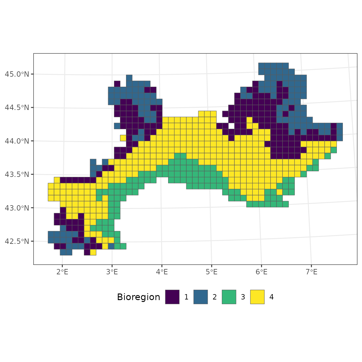
The bioregion 4 is almost constituted of one homogeneous block, which is why the spatial coherence is very close to 100 %.

ggplot(vegemap) +
  geom_sf(aes(fill = as.factor(K_4))) +
  scale_fill_viridis_d("Bioregion") +
  theme_bw() +
  theme(legend.position = "bottom")

5. References

De Cáceres M & Legendre P (2009) Associations between species and groups of sites: Indices and statistical inference. Ecology 90, 3566–3574.

Denelle P, Violle C & Munoz F (2020) Generalist plants are more competitive and more functionally similar to each other than specialist plants: Insights from network analyses. Journal of Biogeography 47, 1922–1933.

Divíšek J, Storch D, Zelený D & Culek M (2016) Towards the spatial coherence of biogeographical regionalizations at subcontinental and landscape scales. Journal of biogeography 43, 2489–2501.

Lenormand M, Papuga G, Argagnon O, Soubeyrand M, Alleaume S & Luque S (2019) Biogeographical network analysis of plant species distribution in the mediterranean region. Ecology and evolution 9, 237–250.

Rousseeuw PJ (1987) Silhouettes: A graphical aid to the interpretation and validation of cluster analysis. Journal of Computational and Applied Mathematics 20, 53–65.

Pierre Denelle, Boris Leroy and Maxime Lenormand

2025-11-12