Hierarchical clustering based on dissimilarity or beta-diversity

This function generates a hierarchical tree from a dissimilarity (beta-diversity) data.frame, calculates the cophenetic correlation coefficient, and optionally retrieves clusters from the tree upon user request. The function includes a randomization process for the dissimilarity matrix to generate the tree, with two methods available for constructing the final tree. Typically, the dissimilarity data.frame is a bioregion.pairwise object obtained by running similarity, or by running similarity followed by similarity_to_dissimilarity.

Usage

hclu_hierarclust(
  dissimilarity,
  index = names(dissimilarity)[3],
  method = "average",
  randomize = TRUE,
  seed = NULL,
  n_runs = 100,
  keep_trials = "no",
  optimal_tree_method = "iterative_consensus_tree",
  n_clust = NULL,
  cut_height = NULL,
  find_h = TRUE,
  h_max = 1,
  h_min = 0,
  consensus_p = 0.5,
  show_hierarchy = FALSE,
  verbose = TRUE
)

Arguments

dissimilarity: The output object from dissimilarity() or similarity_to_dissimilarity(), or a dist object. If a data.frame is used, the first two columns represent pairs of sites (or any pair of nodes), and the subsequent column(s) contain the dissimilarity indices.
index: The name or number of the dissimilarity column to use. By default, the third column name of dissimilarity is used.
method: The name of the hierarchical classification method, as in hclust. Should be one of "ward.D", "ward.D2", "single", "complete", "average" (= UPGMA), "mcquitty" (= WPGMA), "median" (= WPGMC), or "centroid" (= UPGMC).
randomize: A boolean indicating whether the dissimilarity matrix should be randomized to account for the order of sites in the dissimilarity matrix.
seed: A value for the random number generator (NULL for random by default).
n_runs: The number of trials for randomizing the dissimilarity matrix.
keep_trials: A character string indicating whether random trial results (including the randomized matrix, the associated tree and metrics for that tree) should be stored in the output object. Possible values are "no" (default), "all" or "metrics". Note that this parameter is automatically set to "no" if optimal_tree_method = "iterative_consensus_tree".
optimal_tree_method: A character string indicating how the final tree should be obtained from all trials. Possible values are "iterative_consensus_tree" (default), "best" or "consensus". We recommend "iterative_consensus_tree". See Details.
n_clust: An integer vector or a single integer indicating the number of clusters to be obtained from the hierarchical tree, or the output from bioregionalization_metrics. This parameter should not be used simultaneously with cut_height.
cut_height: A numeric vector indicating the height(s) at which the tree should be cut. This parameter should not be used simultaneously with n_clust.
find_h: A boolean indicating whether the height of the cut should be found for the requested n_clust.
h_max: A numeric value indicating the maximum possible tree height for the chosen index.
h_min: A numeric value indicating the minimum possible height in the tree for the chosen index.
consensus_p: A numeric value (applicable only if optimal_tree_method = "consensus") indicating the threshold proportion of trees that must support a region/cluster for it to be included in the final consensus tree.
show_hierarchy: A boolean specifying if the hierarchy of clusters should be identifiable in the outputs (FALSE by default). This argument is only used if the tree is cut (i.e., n_clust or cut_height is provided).
verbose: A boolean indicating whether to display progress messages. Set to FALSE to suppress these messages.

Value

A list of class bioregion.clusters with five slots:

name: A character string containing the name of the algorithm.
args: A list of input arguments as provided by the user.
inputs: A list describing the characteristics of the clustering process.
algorithm: A list containing all objects associated with the clustering procedure, such as the original cluster objects.
clusters: A data.frame containing the clustering results.

In the algorithm slot, users can find the following elements:

trials: A list containing all randomization trials. Each trial includes the dissimilarity matrix with randomized site order, the associated tree, and the cophenetic correlation coefficient for that tree.
final.tree: An hclust object representing the final hierarchical tree to be used.
final.tree.coph.cor: The cophenetic correlation coefficient between the initial dissimilarity matrix and the final.tree.

Details

The function is based on hclust. The default method for the hierarchical tree is average, i.e. UPGMA as it has been recommended as the best method to generate a tree from beta diversity dissimilarity (Kreft & Jetz, 2010).

Clusters can be obtained by two methods:

Specifying a desired number of clusters in n_clust
Specifying one or several heights of cut in cut_height

To find an optimal number of clusters, see bioregionalization_metrics()

It is important to pay attention to the fact that the order of rows in the input distance matrix influences the tree topology as explained in Dapporto (2013). To address this, the function generates multiple trees by randomizing the distance matrix.

Two methods are available to obtain the final tree:

optimal_tree_method = "iterative_consensus_tree": The Iterative Hierarchical Consensus Tree (IHCT) method reconstructs a consensus tree by iteratively splitting the dataset into two subclusters based on the pairwise dissimilarity of sites across n_runs trees based on n_runs randomizations of the distance matrix. At each iteration, it identifies the majority membership of sites into two stable groups across all trees, calculates the height based on the selected linkage method (method), and enforces monotonic constraints on node heights to produce a coherent tree structure. This approach provides a robust, hierarchical representation of site relationships, balancing cluster stability and hierarchical constraints.
optimal_tree_method = "best": This method selects one tree among with the highest cophenetic correlation coefficient, representing the best fit between the hierarchical structure and the original distance matrix.
optimal_tree_method = "consensus": This method constructs a consensus tree using phylogenetic methods with the function consensus. When using this option, you must set the consensus_p parameter, which indicates the proportion of trees that must contain a region/cluster for it to be included in the final consensus tree. Consensus trees lack an inherent height because they represent a majority structure rather than an actual hierarchical clustering. To assign heights, we use a non-negative least squares method (nnls.tree) based on the initial distance matrix, ensuring that the consensus tree preserves approximate distances among clusters.

We recommend using the "iterative_consensus_tree" as all the branches of this tree will always reflect the majority decision among many randomized versions of the distance matrix. This method is inspired by Dapporto et al. (2015), which also used the majority decision among many randomized versions of the distance matrix, but it expands it to reconstruct the entire topology of the tree iteratively.

We do not recommend using the basic consensus method because in many contexts it provides inconsistent results, with a meaningless tree topology and a very low cophenetic correlation coefficient.

For a fast exploration of the tree, we recommend using the best method which will only select the tree with the highest cophenetic correlation coefficient among all randomized versions of the distance matrix.

References

Kreft H & Jetz W (2010) A framework for delineating biogeographical regions based on species distributions. Journal of Biogeography 37, 2029-2053.

Dapporto L, Ramazzotti M, Fattorini S, Talavera G, Vila R & Dennis, RLH (2013) Recluster: an unbiased clustering procedure for beta-diversity turnover. Ecography 36, 1070–1075.

Dapporto L, Ciolli G, Dennis RLH, Fox R & Shreeve TG (2015) A new procedure for extrapolating turnover regionalization at mid-small spatial scales, tested on British butterflies. Methods in Ecology and Evolution 6 , 1287–1297.

Author

Boris Leroy (leroy.boris@gmail.com)
Pierre Denelle (pierre.denelle@gmail.com)
Maxime Lenormand (maxime.lenormand@inrae.fr)

Examples

comat <- matrix(sample(0:1000, size = 500, replace = TRUE, prob = 1/1:1001),
20, 25)
rownames(comat) <- paste0("Site",1:20)
colnames(comat) <- paste0("Species",1:25)

dissim <- dissimilarity(comat, metric = "Simpson")

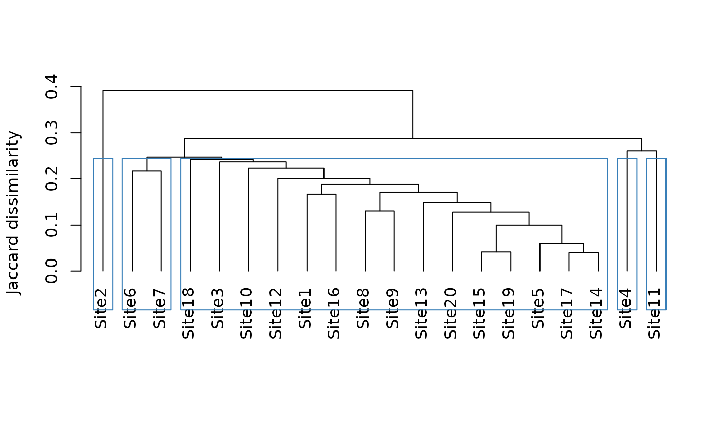
# User-defined number of clusters
tree1 <- hclu_hierarclust(dissim, 
                          n_clust = 5)
#> Building the iterative hierarchical consensus tree... Note that this process can take time especially if you have a lot of sites.
#> 
#> Final tree has a 0.5104 cophenetic correlation coefficient with the initial dissimilarity matrix
#> Determining the cut height to reach 5 groups...
#> --> 0.1171875
tree1
#> Clustering results for algorithm : hclu_hierarclust 
#> 	(hierarchical clustering based on a dissimilarity matrix)
#>  - Number of sites:  20 
#>  - Name of dissimilarity metric:  Simpson 
#>  - Tree construction method:  average 
#>  - Randomization of the dissimilarity matrix:  yes, number of trials 100 
#>  - Method to compute the final tree:  Iterative hierarchical consensus tree 
#>  - Cophenetic correlation coefficient:  0.51 
#>  - Number of clusters requested by the user:  5 
#> Clustering results:
#>  - Number of partitions:  1 
#>  - Number of clusters:  5 
#>  - Height of cut of the hierarchical tree: 0.117 
plot(tree1)

str(tree1)
#> List of 6
#>  $ name        : chr "hclu_hierarclust"
#>  $ args        :List of 16
#>   ..$ index              : chr "Simpson"
#>   ..$ method             : chr "average"
#>   ..$ randomize          : logi TRUE
#>   ..$ seed               : NULL
#>   ..$ n_runs             : num 100
#>   ..$ optimal_tree_method: chr "iterative_consensus_tree"
#>   ..$ keep_trials        : chr "no"
#>   ..$ n_clust            : num 5
#>   ..$ cut_height         : NULL
#>   ..$ find_h             : logi TRUE
#>   ..$ h_max              : num 1
#>   ..$ h_min              : num 0
#>   ..$ consensus_p        : num 0.5
#>   ..$ show_hierarchy     : logi FALSE
#>   ..$ verbose            : logi TRUE
#>   ..$ dynamic_tree_cut   : logi FALSE
#>  $ inputs      :List of 9
#>   ..$ bipartite      : logi FALSE
#>   ..$ weight         : logi TRUE
#>   ..$ pairwise       : logi TRUE
#>   ..$ pairwise_metric: chr "Simpson"
#>   ..$ dissimilarity  : logi TRUE
#>   ..$ nb_sites       : int 20
#>   ..$ data_type      : chr "occurrence"
#>   ..$ node_type      : chr "site"
#>   ..$ hierarchical   : logi FALSE
#>  $ algorithm   :List of 6
#>   ..$ final.tree         :List of 5
#>   .. ..- attr(*, "class")= chr "hclust"
#>   ..$ final.tree.coph.cor: num 0.51
#>   ..$ final.tree.msd     : num 0.00259
#>   ..$ output_n_clust     : int 5
#>   ..$ output_cut_height  : Named num 0.117
#>   .. ..- attr(*, "names")= chr "k_5"
#>   ..$ trials             : chr "Trials not stored in output"
#>  $ clusters    :'data.frame':	20 obs. of  2 variables:
#>   ..$ ID : chr [1:20] "Site1" "Site10" "Site11" "Site12" ...
#>   ..$ K_5: chr [1:20] "1" "1" "1" "1" ...
#>   ..- attr(*, "node_type")= chr [1:20] "site" "site" "site" "site" ...
#>  $ cluster_info:'data.frame':	1 obs. of  4 variables:
#>   ..$ partition_name   : chr "K_5"
#>   ..$ n_clust          : int 5
#>   ..$ requested_n_clust: num 5
#>   ..$ output_cut_height: num 0.117
#>  - attr(*, "class")= chr [1:2] "bioregion.clusters" "list"
tree1$clusters
#>            ID K_5
#> Site1   Site1   1
#> Site10 Site10   1
#> Site11 Site11   1
#> Site12 Site12   1
#> Site13 Site13   1
#> Site14 Site14   1
#> Site15 Site15   1
#> Site16 Site16   1
#> Site17 Site17   2
#> Site18 Site18   1
#> Site19 Site19   1
#> Site2   Site2   3
#> Site20 Site20   1
#> Site3   Site3   1
#> Site4   Site4   4
#> Site5   Site5   1
#> Site6   Site6   4
#> Site7   Site7   4
#> Site8   Site8   1
#> Site9   Site9   5

# User-defined height cut
# Only one height
tree2 <- hclu_hierarclust(dissim, 
                          cut_height = .05)
#> Building the iterative hierarchical consensus tree... Note that this process can take time especially if you have a lot of sites.
#> 
#> Final tree has a 0.5104 cophenetic correlation coefficient with the initial dissimilarity matrix
tree2
#> Clustering results for algorithm : hclu_hierarclust 
#> 	(hierarchical clustering based on a dissimilarity matrix)
#>  - Number of sites:  20 
#>  - Name of dissimilarity metric:  Simpson 
#>  - Tree construction method:  average 
#>  - Randomization of the dissimilarity matrix:  yes, number of trials 100 
#>  - Method to compute the final tree:  Iterative hierarchical consensus tree 
#>  - Cophenetic correlation coefficient:  0.51 
#>  - Heights of cut requested by the user:  0.05 
#> Clustering results:
#>  - Number of partitions:  1 
#>  - Number of clusters:  15 
#>  - Height of cut of the hierarchical tree: 0.05 
tree2$clusters
#>        ID K_15
#> 1   Site1    1
#> 2  Site10    1
#> 3  Site11    2
#> 4  Site12    3
#> 5  Site13    4
#> 6  Site14    5
#> 7  Site15    5
#> 8  Site16    6
#> 9  Site17    7
#> 10 Site18    8
#> 11 Site19    2
#> 12  Site2    9
#> 13 Site20   10
#> 14  Site3   11
#> 15  Site4   12
#> 16  Site5    1
#> 17  Site6   13
#> 18  Site7   14
#> 19  Site8    3
#> 20  Site9   15

# Multiple heights
tree3 <- hclu_hierarclust(dissim, 
                          cut_height = c(.05, .15, .25))
#> Building the iterative hierarchical consensus tree... Note that this process can take time especially if you have a lot of sites.
#> 
#> Final tree has a 0.5104 cophenetic correlation coefficient with the initial dissimilarity matrix

tree3$clusters # Mind the order of height cuts: from deep to shallow cuts
#>            ID K_1 K_3 K_15
#> Site1   Site1   1   1    1
#> Site10 Site10   1   1    1
#> Site11 Site11   1   1    2
#> Site12 Site12   1   1    3
#> Site13 Site13   1   1    4
#> Site14 Site14   1   1    5
#> Site15 Site15   1   1    5
#> Site16 Site16   1   1    6
#> Site17 Site17   1   2    7
#> Site18 Site18   1   1    8
#> Site19 Site19   1   1    2
#> Site2   Site2   1   1    9
#> Site20 Site20   1   1   10
#> Site3   Site3   1   1   11
#> Site4   Site4   1   1   12
#> Site5   Site5   1   1    1
#> Site6   Site6   1   1   13
#> Site7   Site7   1   1   14
#> Site8   Site8   1   1    3
#> Site9   Site9   1   3   15
# Info on each partition can be found in table cluster_info
tree3$cluster_info
#>        partition_name n_clust requested_cut_height
#> h_0.25            K_1       1                 0.25
#> h_0.15            K_3       3                 0.15
#> h_0.05           K_15      15                 0.05
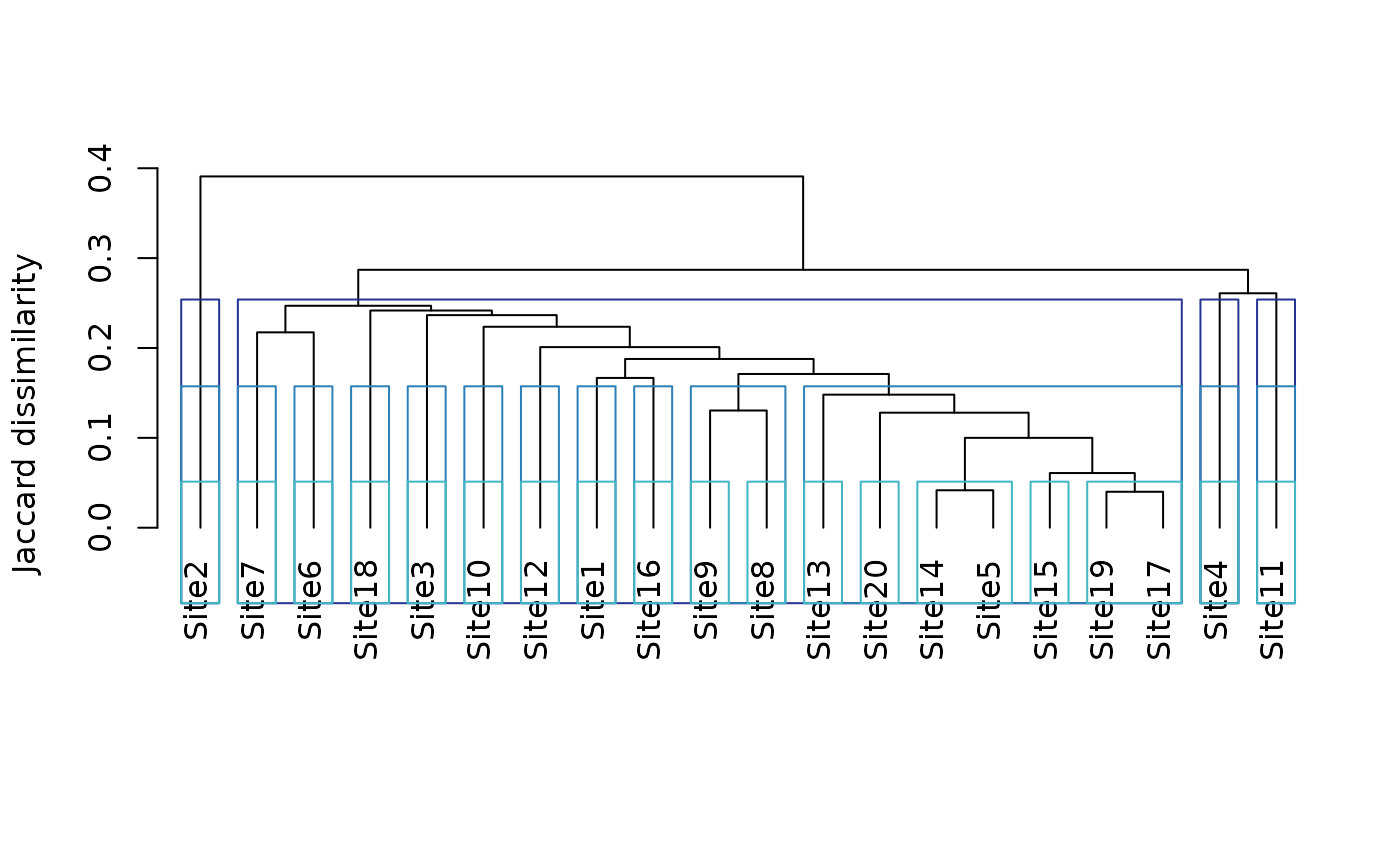
plot(tree3)