4.3 Network clustering

Networks are objects made of nodes and links. The links connect the nodes. Networks can be bipartite, i.e. the nodes can be of two different types and one type can only be linked with the second one. Links can also be weighted.

Site-species matrices can be viewed as bipartite networks where sites and species are two different classes of nodes, and the occurrences of species within sites are the links.

The community detection algorithms try to identify the communities of nodes that interact more with each other than the network as a whole. Appling these algorithms to site-species matrices is therefore equivalent to the more classic bioregionalization methods.

The optimal community partition of a network can be found by searching for the partition that maximizes a metric called modularity. Maximising the modularity is a computationally hard problem requiring the use of algorithms.

Network theory offers plenty of such algorithms to classify nodes that are more connected than expected randomly based or not on the modularity. With the bioregion R package, we cover the main network algorithms to identify bioregions in site-species matrices. All functions relying on network algorithms start with the prefix netclu_.

Network clustering takes place on the left-hand size part of the bioregion conceptual diagram:

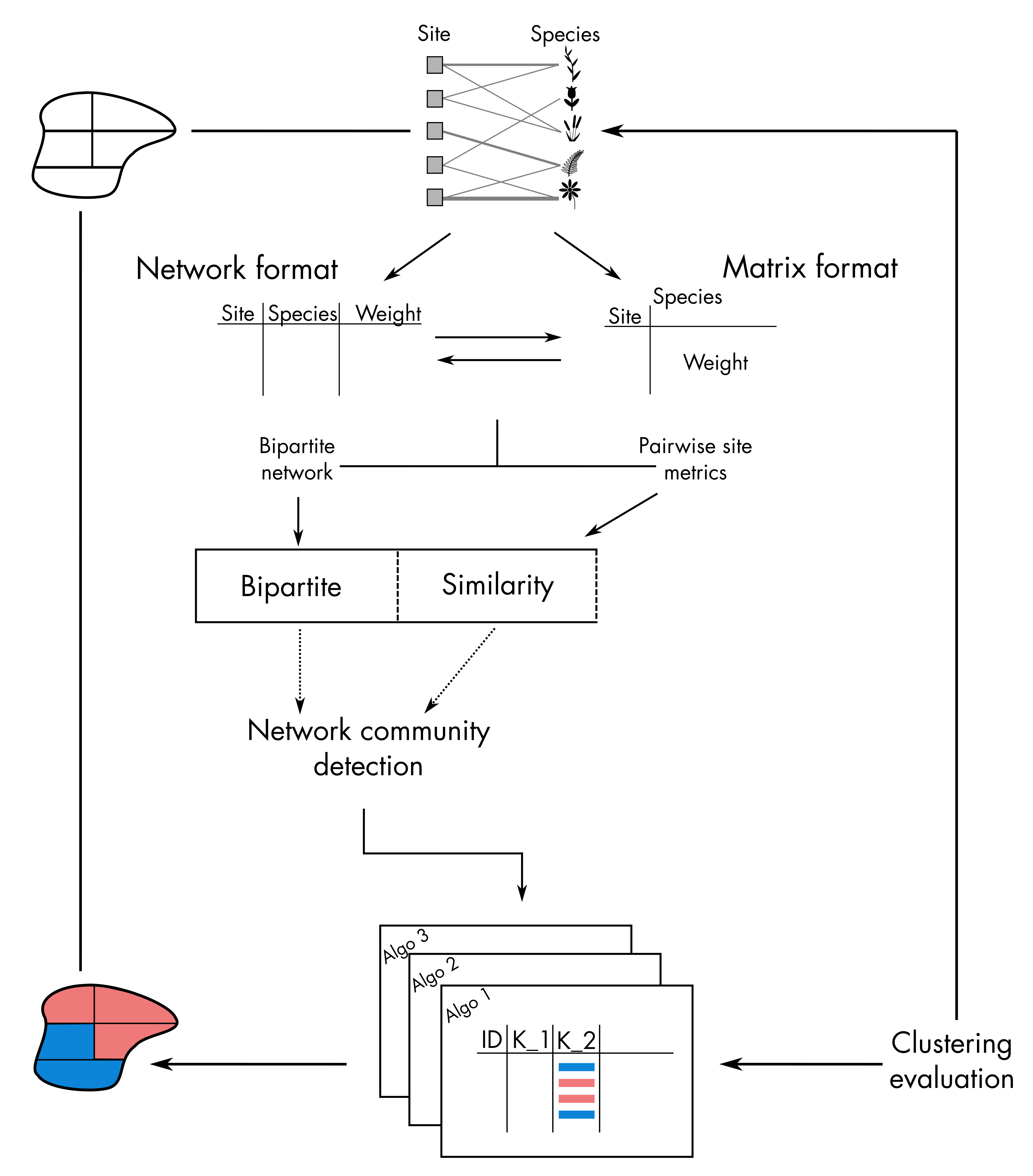
In total, we have 9 functions, which can be classified like this:

Functions based on binary files
netclu_infomap
netclu_oslom
netclu_louvain

- Functions based on the igraph package
* netclu_louvain
* netclu_greedy
* netclu_labelprop
* netclu_leadingeigen
* netclu_walktrap

- Function based on the bipartite package
* netclu_beckett

This vignette aims at briefly explaining how each algorithm and its associated bioregion function works. For this purpose, we use the European freshwater fish dataset that comes with bioregion.

Introduction

Input data

All network algorithms work with the network format, i.e. a data.frame with 3 columns: sites, species and the abundance of a given species in a given site. This type of object can be obtained from a site x species matrix through the use of mat_to_net().

In this vignette, we directly load the network format for the distribution of fish in European basins.

library("bioregion")
data("fishdf")

Some network algorithms work with the similarity matrix between each pair of sites.

data("fishmat")
fish_simil <- similarity(fishmat, metric = "Simpson")

Main arguments

Each of the algorithms presented here has some specific parameters that can be tweaked but some arguments are common for all the functions.

Among these common arguments are the following:
* weight a boolean indicating if the weights should be considered
* index name or number of the column to use as weight. By default, the third column name of the network data.frame is used
* site_col name or number for the column of site nodes (i.e. primary nodes).
* species_col = name or number for the column of species nodes (i.e. feature nodes)
* return_node_type a character indicating what types of nodes (“sites”, “species” or “both”) should be returned in the output (keep_nodes_type=“both” by default).
* algorithm_in_output a boolean indicating if the original output of communities should be returned in the output (see Value).

For the three algorithms relying on executable binary files, the following arguments are needed:
* delete_temp a boolean indicating if the temporary folder should be removed
* path_temp a character indicating the path to the temporary folder
* binpath a character indicating the path to the bin folder

Binary files

install_binaries(binpath = "tempdir", infomap_version = c("2.1.0", "2.6.0"))

Infomap

Rosvall & Bergstrom (2008)

nbmod penalize solutions the more they differ from this number (0 by default for no preferred number of modules).
markovtime scales link flow to change the cost of moving between modules,
higher values results in fewer modules (default is 1).
seed for the random number generator (NULL for random by default)
numtrials the number of trials before picking up the best solution.
twolevel a boolean indicating if the algorithm should optimize a two-level partition of the network (default is multi-level).
show_hierarchy a boolean specifying if the hierarchy of community should be identifiable in the outputs (FALSE by default).

set.seed(1)
ex_infomap <- netclu_infomap(fish_simil,
                             weight = TRUE,
                             index = names(fish_simil)[3],
                             nbmod = 0,
                             markovtime = 1,
                             seed = NULL,
                             numtrials = 1,
                             twolevel = FALSE,
                             show_hierarchy = FALSE,
                             directed = FALSE,
                             bipartite_version = FALSE,
                             bipartite = FALSE,
                             site_col = 1,
                             species_col = 2,
                             return_node_type = "both",
                             version = "2.6.0",
                             binpath = "tempdir",
                             path_temp = "infomap_temp",
                             delete_temp = TRUE)

table(ex_infomap$clusters$K_5)

## 
##   1   2   3   4   5 
## 290  14  23   9   2

OSLOM

OSLOM stands for Order Statistics Local Optimization Method.

Similarity-based algorithm.

Lancichinetti et al. (2011) reassign a string indicating if the nodes belonging to several community should be reassign and what method should be used (see Note).
* r the number of runs for the first hierarchical level (10 by default).
* hr the number of runs for the higher hierarchical level (50 by default, 0 if you are not interested in hierarchies).
* seed for the random number generator (NULL for random by default).
* t the p-value, the default value is 0.10, increase this value you to get more modules.
* cp kind of resolution parameter used to decide between taking some modules or their union (default value is 0.5, bigger value leads to bigger clusters).

set.seed(1)
ex_oslom <- netclu_oslom(fish_simil,
                         weight = TRUE,
                         index = names(fish_simil)[3],
                         reassign = "no",
                         r = 10,
                         hr = 50,
                         seed = NULL,
                         t = 0.1,
                         cp = 0.5,
                         directed = FALSE,
                         bipartite = FALSE,
                         site_col = 1,
                         species_col = 2,
                         return_node_type = "both",
                         binpath = "tempdir",
                         path_temp = "oslom_temp",
                         delete_temp = TRUE)

table(ex_oslom$clusters$K_338)

Louvain

Blondel et al. (2008)

q the quality function used to compute partition of the graph (modularity is chosen by default, see Details).
c the parameter for the Owsinski-Zadrozny quality function (between 0 and 1, 0.5 is chosen by default)
k the kappa_min value for the Shi-Malik quality function (it must be > 0, 1 is chosen by default)

set.seed(1)
ex_louvain <- netclu_louvain(fishdf,
                             weight = TRUE,
                             index = names(fishdf)[3],
                             lang = "cpp",
                             q = 0,
                             c = 0.5,
                             k = 1,
                             bipartite = FALSE,
                             site_col = 1,
                             species_col = 2,
                             return_node_type = "both",
                             binpath = "tempdir",
                             path_temp = "louvain_temp",
                             delete_temp = TRUE,
                             algorithm_in_output = TRUE)
table(ex_louvain$clusters$K_23)

## 
##   1  10  11  12  13  14  15  16  17  18  19   2  20  21  22  23   3   4   5   6 
##  17   3  21 113   6  44  98  55   5  52   3  10   4  16   2   4  10  22   5   4 
##   7   8   9 
##   3  11  25

Functions from the igraph package

Fastgreedy

Clauset et al. (2004)

set.seed(1)
ex_greedy <- netclu_greedy(fishdf,
                           weight = TRUE,
                           index = names(fishdf)[3],
                           bipartite = FALSE,
                           site_col = 1,
                           species_col = 2,
                           return_node_type = "both",
                           algorithm_in_output = TRUE)
table(ex_greedy$clusters$K_5)

## 
##   1   2   3   4   5 
## 138  61 144 132  58

Label propagation

Raghavan et al. (2007)

set.seed(1)
ex_labelprop <- netclu_labelprop(fishdf,
                                 weight = TRUE,
                                 index = names(fishdf)[3],
                                 bipartite = FALSE,
                                 site_col = 1,
                                 species_col = 2,
                                 return_node_type = "both",
                                 algorithm_in_output = TRUE)
table(ex_labelprop$clusters$K_11)

## < table of extent 0 >

Leiden algorithm

Traag et al. (2019)

set.seed(1)
ex_leiden <- netclu_leiden(fishdf,
                           weight = TRUE,
                           index = names(fishdf)[3],
                           objective_function = "CPM",
                           resolution_parameter = 1,
                           beta = 0.01,
                           n_iterations = 2,
                           vertex_weights = NULL,
                           bipartite = TRUE,
                           site_col = 1,
                           species_col = 2,
                           return_node_type = "both",
                           algorithm_in_output = TRUE)
length(unique(ex_leiden$clusters$K_505))

## [1] 0

Leading eigenvector

Newman (2006)

set.seed(1)
ex_leadingeigen <- netclu_leadingeigen(fishdf,
                                       weight = TRUE,
                                       index = names(fishdf)[3],
                                       bipartite = FALSE,
                                       site_col = 1,
                                       species_col = 2,
                                       return_node_type = "both",
                                       algorithm_in_output = TRUE)
table(ex_leadingeigen$clusters$K_17)

## < table of extent 0 >

Walktrap

Pons & Latapy (2005)

set.seed(1)
ex_walktrap <- netclu_walktrap(fishdf,
                               weight = TRUE,
                               index = names(fishdf)[3],
                               steps = 4,
                               bipartite = FALSE,
                               site_col = 1,
                               species_col = 2,
                               return_node_type = "both",
                               algorithm_in_output = TRUE)
table(ex_walktrap$clusters$K_14)

## 
##   1  10  11  12  13  14   2   3   4   5   6   7   8   9 
##  11  47  10   2   6  17  84   5  37  16   5 270   4  19

Function from the bipartite package

Beckett

Update of the QuanBiMo algorithm developed by Dormann & Strauss (2014).

Beckett (2016)

set.seed(1)
ex_beckett <- netclu_beckett(fishdf,
                             weight = TRUE,
                             index = names(fishdf)[3],
                             site_col = 1,
                             species_col = 2,
                             return_node_type = "both",
                             forceLPA = TRUE,
                             algorithm_in_output = TRUE)
ex_beckett$clusters$K_23

##   [1] "4"  "1"  "2"  "3"  "4"  "4"  "3"  "3"  "16" "13" "1"  "1"  "8"  "1"  "16"
##  [16] "5"  "4"  "3"  "4"  "8"  "4"  "1"  "4"  "4"  "5"  "4"  "4"  "1"  "13" "1" 
##  [31] "4"  "3"  "1"  "3"  "4"  "4"  "4"  "4"  "3"  "3"  "4"  "3"  "1"  "5"  "3" 
##  [46] "3"  "6"  "4"  "3"  "4"  "1"  "4"  "1"  "4"  "4"  "4"  "7"  "8"  "4"  "9" 
##  [61] "4"  "4"  "4"  "4"  "10" "10" "1"  "4"  "5"  "1"  "5"  "4"  "8"  "8"  "4" 
##  [76] "1"  "3"  "1"  "16" "13" "12" "1"  "22" "4"  "3"  "1"  "3"  "1"  "13" "4" 
##  [91] "4"  "8"  "4"  "8"  "15" "15" "15" "15" "4"  "1"  "8"  "4"  "1"  "8"  "4" 
## [106] "8"  "4"  "1"  "1"  "4"  "1"  "15" "1"  "1"  "5"  "1"  "16" "8"  "1"  "1" 
## [121] "1"  "13" "1"  "8"  "1"  "8"  "17" "18" "1"  "1"  "1"  "8"  "1"  "19" "1" 
## [136] "1"  "8"  "4"  "4"  "4"  "4"  "5"  "4"  "1"  "1"  "1"  "4"  "4"  "5"  "5" 
## [151] "3"  "8"  "1"  "11" "1"  "4"  "1"  "1"  "1"  "1"  "13" "16" "4"  "1"  "1" 
## [166] "1"  "1"  "1"  "1"  "3"  "8"  "5"  "5"  "20" "5"  "4"  "3"  "1"  "4"  "1" 
## [181] "4"  "1"  "6"  "1"  "13" "3"  "8"  "8"  "4"  "3"  "1"  "8"  "1"  "4"  "8" 
## [196] "1"  "3"  "4"  "1"  "4"  "8"  "4"  "1"  "1"  "4"  "1"  "16" "1"  "4"  "8" 
## [211] "1"  "3"  "15" "1"  "1"  "16" "13" "1"  "3"  "1"  "1"  "1"  "3"  "1"  "21"
## [226] "1"  "4"  "1"  "1"  "1"  "1"  "1"  "4"  "1"  "1"  "1"  "8"  "4"  "4"  "4" 
## [241] "1"  "22" "1"  "1"  "1"  "4"  "1"  "5"  "1"  "4"  "1"  "1"  "1"  "8"  "15"
## [256] "4"  "1"  "4"  "4"  "1"  "4"  "4"  "4"  "8"  "3"  "4"  "8"  "3"  "4"  "1" 
## [271] "1"  "13" "1"  "4"  "22" "1"  "1"  "3"  "3"  "5"  "5"  "4"  "4"  "1"  "4" 
## [286] "4"  "4"  "4"  "3"  "11" "4"  "3"  "4"  "1"  "1"  "1"  "1"  "8"  "4"  "4" 
## [301] "4"  "4"  "3"  "1"  "5"  "1"  "1"  "4"  "5"  "8"  "1"  "1"  "1"  "1"  "1" 
## [316] "5"  "1"  "4"  "1"  "1"  "14" "10" "8"  "4"  "1"  "4"  "4"  "4"  "4"  "3" 
## [331] "1"  "1"  "5"  "4"  "8"  "8"  "4"  "23" "4"  "4"  "4"  "8"  "8"  "1"  "4" 
## [346] "4"  "4"  "13" "1"  "4"  "4"  "1"  "16" "16" "2"  "16" "2"  "2"  "2"  "16"
## [361] "2"  "16" "3"  "4"  "3"  "3"  "3"  "3"  "3"  "3"  "3"  "3"  "4"  "5"  "4" 
## [376] "4"  "3"  "3"  "12" "16" "13" "13" "13" "13" "13" "13" "13" "13" "13" "13"
## [391] "13" "13" "13" "8"  "8"  "16" "16" "5"  "20" "15" "5"  "5"  "4"  "3"  "3" 
## [406] "8"  "15" "5"  "5"  "5"  "5"  "5"  "5"  "13" "8"  "13" "9"  "3"  "3"  "3" 
## [421] "5"  "6"  "19" "6"  "6"  "7"  "7"  "7"  "7"  "7"  "8"  "7"  "7"  "7"  "7" 
## [436] "21" "21" "7"  "21" "7"  "7"  "7"  "7"  "7"  "7"  "8"  "10" "8"  "10" "9" 
## [451] "9"  "9"  "9"  "10" "9"  "9"  "8"  "10" "22" "9"  "9"  "9"  "10" "9"  "8" 
## [466] "10" "9"  "9"  "4"  "10" "10" "8"  "10" "10" "15" "5"  "5"  "11" "11" "15"
## [481] "13" "13" "22" "22" "13" "22" "12" "12" "22" "13" "13" "15" "15" "14" "15"
## [496] "15" "15" "15" "15" "5"  "16" "17" "18" "18" "18" "18" "23" "19" "19" "13"
## [511] "20" "13" "22" "13" "13" "13" "3"  "21" "21" "21" "21" "21" "21" "4"  "22"
## [526] "22" "5"  "22" "22" "22" "5"  "10" "23"

References

Beckett, S. J. (2016). Improved community detection in weighted bipartite networks. Royal Society Open Science, 3(1), 140536.

Blondel, V. D., Guillaume, J. L., Lambiotte, R., & Mech, E. L. J. S. (2008). Fast unfolding of communities in large networks. J. Stat. Mech, 2008(10), P10008.

Clauset, A., Newman, M. E. J., & Moore, C. (2004). Finding community structure in very large networks. Phys. Rev. E, 70, 066111.

Lancichinetti, A., Radicchi, F., Ramasco, J. J., & Fortunato, S. (2011). Finding statistically significant communities in networks. PLOS ONE, 6(4), e18961.

Newman, M. E. J. (2006). Finding community structure in networks using the eigenvectors of matrices. Physical Review E, 74(3), 036104.

Pons, P., & Latapy, M. (2005). Computing Communities in Large Networks Using Random Walks. In I. Yolum, T. Güngör, F. Gürgen, & C. Özturan (Eds.), Computer and Information Sciences - ISCIS 2005 (pp. 284–293). Springer.

Raghavan, U. N., Albert, R., & Kumara, S. (2007). Near linear time algorithm to detect community structures in large-scale networks. Physical Review E, 76(3), 036106.

Rosvall, M., & Bergstrom, C. T. (2008). Maps of random walks on complex networks reveal community structure. Proceedings of the National Academy of Sciences, 105(4), 1118–1123.

Traag, V. A., Waltman, L., & Van Eck, N. J. (2019). From Louvain to Leiden: Guaranteeing well-connected communities. Scientific Reports, 9(1), 5233.

Pierre Denelle, Boris Leroy and Maxime Lenormand

2024-12-16