Tutorial for bioregion

Maxime Lenormand, Boris Leroy and Pierre Denelle

2024-04-19

0. Brief introduction

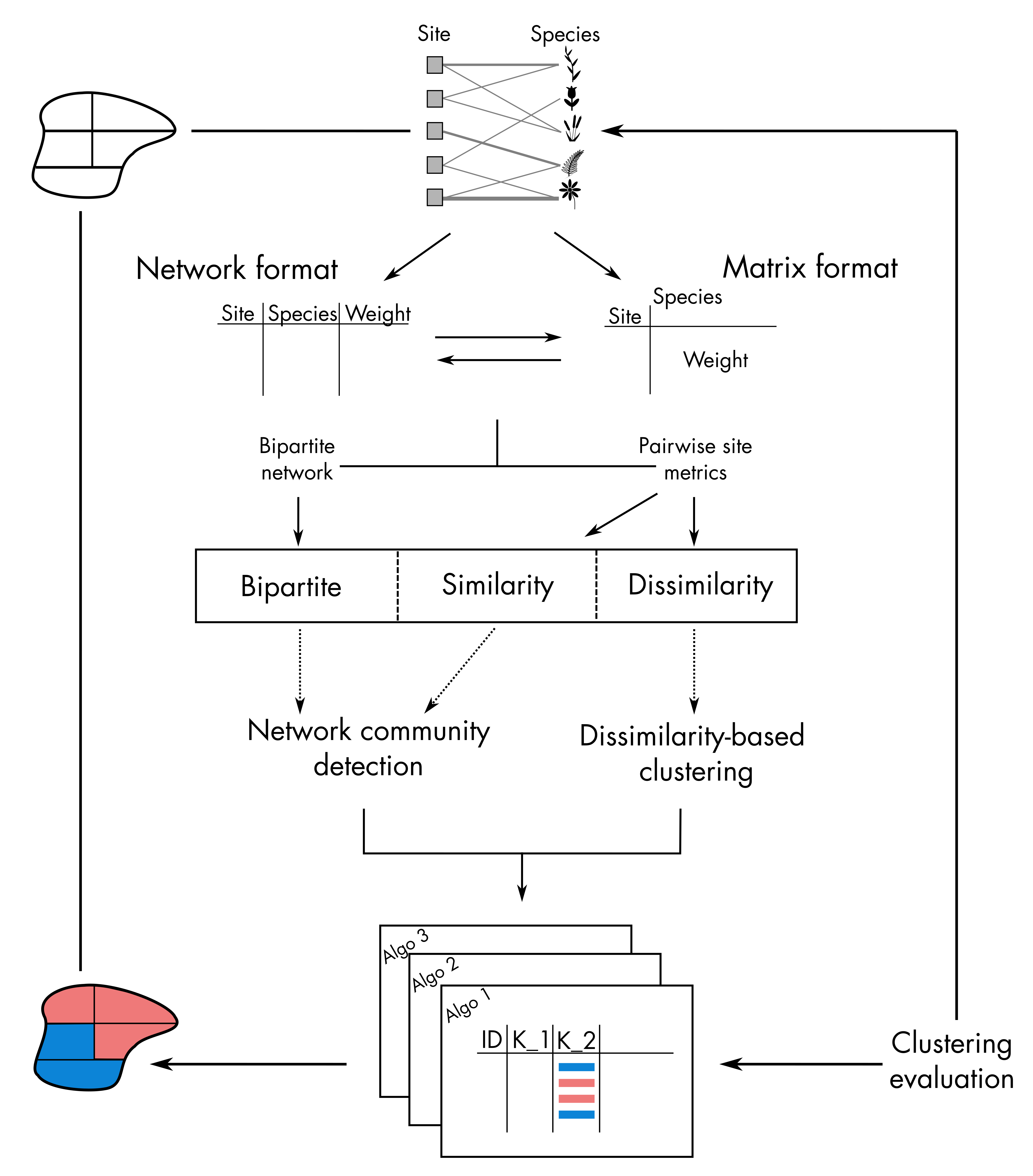
This tutorial aims at describing the different features of the R package bioregion. The main purpose of the bioregion‘s package is to propose a transparent methodological framework to compare bioregionalisation methods. Below is the typical flow chart of bioregions’ identification based on a site-species bipartite network or co-occurrence matrix with bioregion (Figure 1). This workflow can be divided into four main steps:

1. Preprocess the data (matrix or network formats)
2. Compute similarity/dissimilarity metrics between sites based on species composition
3. Run the different algorithms to identify different set of bioregions
4. Evaluate and visualize the results

Figure 1: Workflow of the bioregion’s package.

1. Install binary files

Some functions or at least part of them (listed below) require binary files to run.

• netclu_infomap
• netclu_louvain (Cpp version)
• netclu_oslom

Please check this tutorial page to get instructions regarding the installation of the binary files.

2. Matrix or Network formats

The bioregion’s package takes as input site-species information stored in a bipartite network or a co-occurrence matrix. Relying on the function mat_to_net and net_to_mat , it handles both the matrix and network formats throughout the workflow.

Please have a look at this tutorial page to better understand how these two functions work.

3. Pairwise similarity/dissimilarity metrics

The functions similarity and dissimilarity compute respectively pairwise similarity and dissimilarity metrics based on a (site-species) co-occurrence matrix. The resulting data.frame is stored in a bioregion.pairwise.metric object containing all requested metrics between each pair of sites.

The functions dissimilarity_to_similarity and similarity_to_dissimilarity can be used to transform a similarity object into a dissimilarity object and vice versa.

Please have a look at this tutorial page to better understand how these functions work.

4. Clustering algorithms

The bioregion R package gathers several methods allowing to group sites and species into similar entities called bioregions. All these methods can lead to several partitions of sites and species, i.e. to different bioregionalisations.
Bioregionalisation methods can be based on hierarchical clustering algorithms, non-hierarchical clustering algorithms or network algorithms.
The functions in the package are related to each of these three families and produce output that have a specific class, namely the bioregion.clusters class.

4.1 Hierarchical clustering

The functions relying on hierarchical clustering start with the prefix hclu_. With these algorithms, the bioregions are placed into a dendrogram that ranges from two extremes: all sites belong to the same bioregion (top of the tree) or all sites belong to a different bioregion (bottom of the tree).

See the following tutorial page for more details.

4.2 Non-hierarchical clustering

The functions relying on hierarchical clustering start with the prefix nhclu_. For most of these algorithms, the user needs to predefine the number of clusters, although this number can be determined by estimating the optimal partition.

See this tutorial page for more details.

4.3 Network clustering

The functions relying on network clustering start with the prefix netclu_. Site-species matrices can be seen as (bipartite) networks where the nodes are either the sites or the species and the links between them are the occurrences of species within sites.
With networks, modularity algorithms can be applied, leading to bioregionalisation.

The following tutorial page details more each clustering functions relying on a network algorithm.

4.4 Microbenchmark

The different bioregionalisation methods listed in the package rely on more or less computationally intensive algorithms.

The following page estimates the time required to run each method on data sets of different sizes.

5. Visualization and evaluation of the results

5.1 Visualization

If sites have geographic coordinates, then each bioregionalisation can be visualized with the function map_clusters().

This tutorial page details different ways to plot your bioregionalisation.

5.2 Compare partitions

In this section, we look at how sites are assigned to bioregions within a single bioregionalization and also compare this assignment across different bioregionalizations. The following page illustrates this.