OPTICS hierarchical clustering algorithm

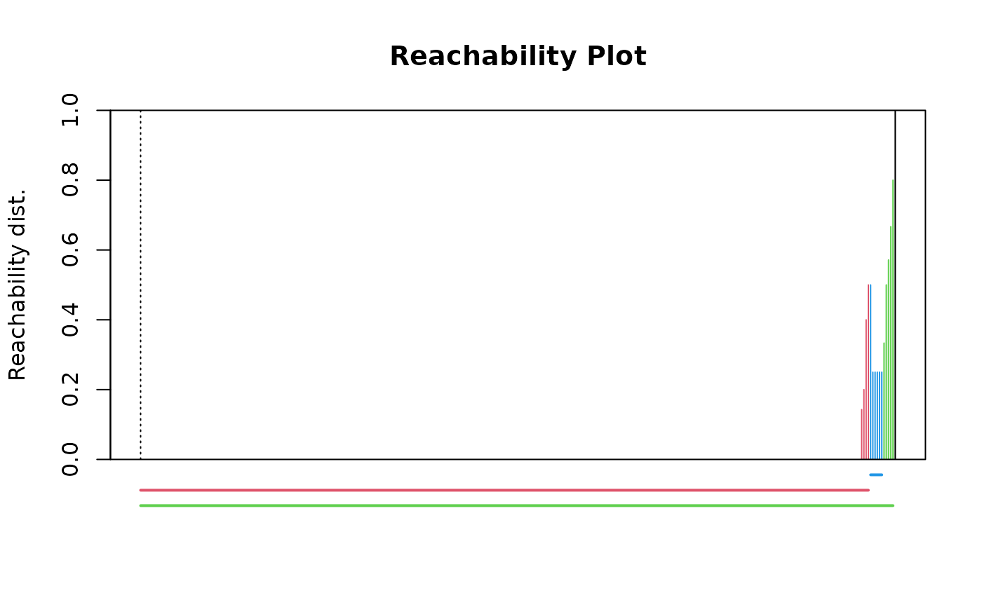
This function performs semi-hierarchical clustering based on dissimilarity using the OPTICS algorithm (Ordering Points To Identify the Clustering Structure).

Usage

hclu_optics(
  dissimilarity,
  index = names(dissimilarity)[3],
  minPts = NULL,
  eps = NULL,
  xi = 0.05,
  minimum = FALSE,
  show_hierarchy = FALSE,
  algorithm_in_output = TRUE,
  ...
)

Arguments

dissimilarity

The output object from dissimilarity() or similarity_to_dissimilarity(), or a dist object. If a data.frame is used, the first two columns represent pairs of sites (or any pair of nodes), and the subsequent column(s) contain the dissimilarity indices.

index

The name or number of the dissimilarity column to use. By default, the third column name of dissimilarity is used.

minPts

A numeric value specifying the minPts argument of dbscan. minPts is the minimum number of points required to form a dense region. By default, it is set to the natural logarithm of the number of sites in dissimilarity.

eps

A numeric value specifying the eps argument of optics. It defines the upper limit of the size of the epsilon neighborhood. Limiting the neighborhood size improves performance and has no or very little impact on the ordering as long as it is not set too low. If not specified (default behavior), the largest minPts-distance in the dataset is used, which gives the same result as infinity.

xi

A numeric value specifying the steepness threshold to identify clusters hierarchically using the Xi method (see optics).

minimum

A boolean specifying whether the hierarchy should be pruned from the output to only retain clusters at the "minimal" level, i.e., only leaf / non-overlapping clusters. If TRUE, then the argument show_hierarchy should be set to FALSE.

show_hierarchy

A boolean specifying whether the hierarchy of clusters should be included in the output. By default, the hierarchy is not visible in the clusters obtained from OPTICS; it can only be visualized by plotting the OPTICS object. If show_hierarchy = TRUE, the output cluster data.frame will contain additional columns showing the hierarchy of clusters.

algorithm_in_output

A boolean indicating whether the original output of dbscan should be returned in the output (TRUE by default, see Value).

...

Additional arguments to be passed to optics() (see optics).

Value

A list of class bioregion.clusters with five slots:

1. name: A character string containing the name of the algorithm.

2. args: A list of input arguments as provided by the user.

3. inputs: A list describing the characteristics of the clustering process.

4. algorithm: A list containing all objects associated with the clustering procedure, such as the original cluster objects.

5. clusters: A data.frame containing the clustering results.

In the algorithm slot, if algorithm_in_output = TRUE, users can find the output of optics.

Details

The OPTICS (Ordering points to identify the clustering structure) is a semi-hierarchical clustering algorithm which orders the points in the dataset such that points which are closest become neighbors, and calculates a reachability distance for each point. Then, clusters can be extracted in a hierarchical manner from this reachability distance, by identifying clusters depending on changes in the relative cluster density. The reachability plot should be explored to understand the clusters and their hierarchical nature, by running plot on the output of the function if algorithm_in_output = TRUE: plot(object$algorithm). We recommend reading (Hahsler et al., 2019) to grasp the algorithm, how it works, and what the clusters mean.

To extract the clusters, we use the extractXi function which is based on the steepness of the reachability plot (see optics)

References

Hahsler M, Piekenbrock M & Doran D (2019) Dbscan: Fast density-based clustering with R. Journal of Statistical Software 91, 1–30.

See also

For more details illustrated with a practical example, see the vignette: https://biorgeo.github.io/bioregion/articles/a4_1_hierarchical_clustering.html.

Associated functions: nhclu_dbscan

Author

Boris Leroy (leroy.boris@gmail.com)
Pierre Denelle (pierre.denelle@gmail.com)
Maxime Lenormand (maxime.lenormand@inrae.fr)

Examples

dissim <- dissimilarity(fishmat, metric = "all")
  
clust1 <- hclu_optics(dissim, index = "Simpson")
clust1
#> Clustering results for algorithm : hclu_optics 
#>  - Number of sites:  338 
#> Clustering results:
#>  - Number of partitions:  1 
#>  - Number of clusters:  4 

# Visualize the optics plot (the hierarchy of clusters is illustrated at the
# bottom)
plot(clust1$algorithm)


# Extract the hierarchy of clusters
clust1 <- hclu_optics(dissim, index = "Simpson", show_hierarchy = TRUE)
clust1
#> Clustering results for algorithm : hclu_optics 
#>  - Number of sites:  338 
#> Clustering results:
#>  - Number of partitions:  2 
#>  - Partitions are hierarchical
#>  - Number of clusters:  2 4