5.1 Visualization
Pierre Denelle, Boris Leroy and Maxime Lenormand
2024-04-19
Source:vignettes/a5_1_visualization.Rmd
a5_1_visualization.RmdIn this vignette, we aim at illustrating how to plot the bioregions
identified with the diferent algorithms available in
bioregion.
Using one of the dataset coming along with
bioregion, we show three strategies to plot your
results.
Data
For this vignette, we rely on the dataset describing the distribution of vascular plants in the Mediterranean part of France. We first load the matrix format of this dataset, computes the dissimilarity matrix out of it and also load the data.frame format of the data.
data(vegemat)
vegedissim <- dissimilarity(vegemat, metric = "all")
data(vegedf)
Since we aim at plotting the result, we also need the object
fishsf linking each site of the dataset to a geometry.
data(vegesf)We also import the world coastlines, available from the
rnaturalearth R package.
world <- rnaturalearth::ne_coastline(returnclass = "sf", scale = "medium")
# Align the CRS of both objects
vegesf <- st_transform(vegesf, crs = st_crs(world))
Plots
In this section, we show three ways to plot your results.
map_clusters()
The first possibility is to use the function
map_clusters() from the package. This function can directly
provide a plot of each site colored according to the cluster they belong
to.
Let’s take an example with a K-means clustering, with a number
of clusters set to 3.
vege_nhclu_kmeans <- nhclu_kmeans(vegedissim, n_clust = 3, index = "Simpson")map_clusters() function can now simply takes the object
fish_nhclu_kmeans, which is of
bioregion.clusters class, and the spatial distribution of
sites, stored in fishsf.
map_clusters(vege_nhclu_kmeans, geometry = vegesf, plot = TRUE)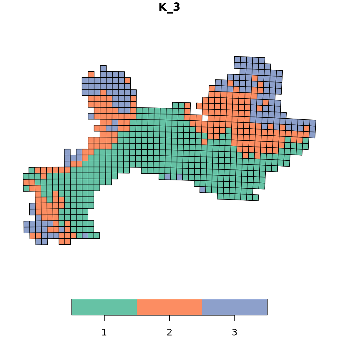
Custom plot
If you want to customize yourself the plot and not simply rely on the
default option, map_clusters() gives you the possibility to
extract each site as well as its geometry and cluster number.
For this purpose, you can set the arguments like in the chunk below:
custom <- map_clusters(vege_nhclu_kmeans, geometry = vegesf,
                       write_clusters = TRUE, plot = FALSE)
custom
## Simple feature collection with 715 features and 2 fields
## Geometry type: POLYGON
## Dimension: XY
## Bounding box: xmin: 1.686171 ymin: 42.29604 xmax: 7.798711 ymax: 45.13742
## Geodetic CRS: WGS 84
## First 10 features:
## ID K_3 geometry
## 1 35 3 POLYGON ((6.098099 45.13742...
## 2 36 3 POLYGON ((6.22521 45.13381,...
## 3 37 3 POLYGON ((6.352304 45.13007...
## 4 38 3 POLYGON ((6.47938 45.12617,...
## 5 39 3 POLYGON ((6.606438 45.12213...
## 6 84 3 POLYGON ((6.093117 45.04745...
## 7 85 3 POLYGON ((6.220024 45.04385...
## 8 86 3 POLYGON ((6.346914 45.04011...
## 9 87 3 POLYGON ((6.473786 45.03622...
## 10 88 3 POLYGON ((6.600641 45.03219...
# Crop world coastlines to the extent of the sf object of interest
europe <- sf::st_crop(world, sf::st_bbox(custom))

# Plot
ggplot(custom) +
  geom_sf(aes(fill = K_3), show.legend = FALSE) +
  geom_sf(data = europe) +
  scale_fill_viridis_d() +
  labs(title = "Kmeans with 3 clusters") +
  theme_void()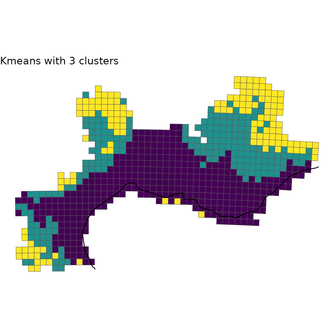
Plot with facets
Finally, you can be interested in plotting several
bioregionalisations at once. For this purpose, we can build a single
data.frame gathering all the bioregions obtained from
distinct algorithms and then take advantage of the facets
implemented in ggplot2.
We first compute a few more bioregionalisation on the same dataset
using other algorithms.
# Hierarchical clustering
set.seed(1)
vege_hclu_hierarclust <- hclu_hierarclust(dissimilarity = vegedissim,
                                          index = names(vegedissim)[6],
                                          method = "mcquitty", n_clust = 3)
vege_hclu_hierarclust$cluster_info
## partition_name n_clust requested_n_clust output_cut_height
## 1 K_3 3 3 0.625
# Walktrap network bioregionalization
vegesim <- dissimilarity_to_similarity(vegedissim)
set.seed(1)
vege_netclu_walktrap <- netclu_walktrap(vegesim,
                                        index = names(vegesim)[6])
vege_netclu_walktrap$cluster_info # 3
## partition_name n_clust
## K_3 K_3 3We can now make a single data.frame with an extra-column
indicating the algorithm used.
vege_kmeans <- vege_nhclu_kmeans$clusters
colnames(vege_kmeans)<- c("ID", "NHCLU_KMEANS")
vege_hieraclust <- vege_hclu_hierarclust$clusters
colnames(vege_hieraclust)<- c("ID", "HCLU_HIERARCLUST")
vege_walktrap <- vege_netclu_walktrap$clusters
colnames(vege_walktrap)<- c("ID", "NETCLU_Walktrap")

all_clusters <- dplyr::left_join(vege_kmeans, vege_hieraclust, by = "ID")
all_clusters <- dplyr::left_join(all_clusters, vege_walktrap, by = "ID")
We now convert this data.frame into a long-format
data.frame.
all_long <- tidyr::pivot_longer(data = all_clusters,
                                cols = dplyr::contains("_"),
                                names_to = "Algorithm",
                                values_to = "Clusters")
all_long <- as.data.frame(all_long)
We now add back the geometry as an extra column to make this object spatial.
all_long_sf <- dplyr::left_join(all_long,
                                vegesf[, c("ID", "geometry")],
                                by = "ID")
all_long_sf <- sf::st_as_sf(all_long_sf)
Now that we have a long-format spatial data.frame, we
can take advantage of the facets implemented in
ggplot2.
ggplot(all_long_sf) +
  geom_sf(aes(color = Clusters, fill = Clusters)) +
  geom_sf(data = europe, fill = "gray80") +
  scale_color_viridis_d() +
  scale_fill_viridis_d() +
  theme_void() +
  facet_wrap(~ Algorithm)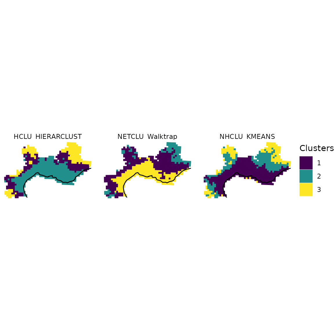
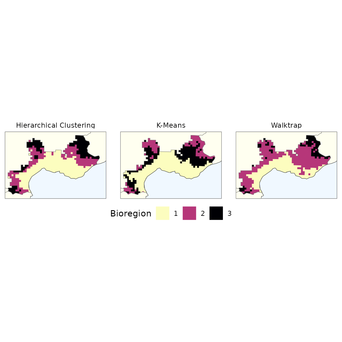
We can refine the above map by: * reordering the 3 bioregions so that they follow the same order * add some background for the Mediterranean sea and the mainland * crop the cells by the mainland * adjust labels
world_countries <- rnaturalearth::ne_countries(scale = "medium",
                                               returnclass = "sf")

# Background box
xmin <- st_bbox(world)[["xmin"]]; xmax <- st_bbox(world)[["xmax"]]
ymin <- st_bbox(world)[["ymin"]]; ymax <- st_bbox(world)[["ymax"]]
bb <- sf::st_union(sf::st_make_grid(st_bbox(c(xmin = xmin,
                                              xmax = xmax,
                                              ymax = ymax,
                                              ymin = ymin),
                                            crs = st_crs(4326)),
                                    n = 100))

# Crop world coastlines to the extent of the sf object of interest
vegesf <- st_transform(vegesf, crs = st_crs(world))
larger_bbox <- sf::st_bbox(vegesf)
larger_bbox[[1]] <- 1.5
larger_bbox[[2]] <- 42.15
larger_bbox[[3]] <- 8.1
larger_bbox[[4]] <- 45.3

europe <- sf::st_crop(world, larger_bbox)
sf_use_s2(FALSE)
europe_countries <- sf::st_crop(world_countries, larger_bbox)
europe_bb <- sf::st_crop(bb, larger_bbox)

plot_basis <- ggplot(europe) +
  geom_sf(data = europe_bb, fill = "aliceblue") +
  geom_sf(data = europe_countries, fill = "ivory", color = "gray50") +
  theme_void()

# Reordering bioregions
all_long_sf$bioregion <- all_long_sf$Clusters

all_long_sf[which(all_long_sf$Algorithm == "HCLU_HIERARCLUST" &
                    all_long_sf$Clusters == "2"), ]$bioregion <- "1"
all_long_sf[which(all_long_sf$Algorithm == "HCLU_HIERARCLUST" &
                    all_long_sf$Clusters == "1"), ]$bioregion <- "2"

all_long_sf[which(all_long_sf$Algorithm == "NHCLU_KMEANS" &
                    all_long_sf$Clusters == "3"), ]$bioregion <- "2"
all_long_sf[which(all_long_sf$Algorithm == "NHCLU_KMEANS" &
                    all_long_sf$Clusters == "1"), ]$bioregion <- "1"
all_long_sf[which(all_long_sf$Algorithm == "NHCLU_KMEANS" &
                    all_long_sf$Clusters == "2"), ]$bioregion <- "3"

all_long_sf[which(all_long_sf$Algorithm == "NETCLU_Walktrap" &
                    all_long_sf$Clusters == "3"), ]$bioregion <- "1"
all_long_sf[which(all_long_sf$Algorithm == "NETCLU_Walktrap" &
                    all_long_sf$Clusters == "1"), ]$bioregion <- "2"
all_long_sf[which(all_long_sf$Algorithm == "NETCLU_Walktrap" &
                    all_long_sf$Clusters == "2"), ]$bioregion <- "3"

# More readable labels for algorithms
all_long_sf$Algo <-
  ifelse(all_long_sf$Algorithm == "NHCLU_KMEANS", "K-Means",
         ifelse(all_long_sf$Algorithm == "NHCLU_PAM", "PAM",
                ifelse(all_long_sf$Algorithm == "HCLU_HIERARCLUST",
                       "Hierarchical Clustering", "Walktrap")))

# Cropping with borders of France
all_long_sf_france <-
  st_intersection(all_long_sf,
                  europe_countries[which(europe_countries$sovereignt == "France"), ])

# Plot
final_plot <- plot_basis +
  geom_sf(data = all_long_sf_france,
          aes(color = bioregion, fill = bioregion), show.legend = TRUE) +
  geom_sf(data = st_union(all_long_sf_france), fill = "NA", color = "gray50") +
  geom_sf(data = europe, fill = "gray50", linewidth = 0.1) +
  scale_color_viridis_d("Bioregion", option = "magma", direction = -1) +
  scale_fill_viridis_d("Bioregion", option = "magma", direction = -1) +
  theme_void() +
  theme(legend.position = "bottom") +
  facet_wrap(~ Algo)
final_plot