4.4 Microbenchmark

In this vignette, we aim at showing the differences in terms of computation time between the different algorithms available in bioregion. For this purpose, we use three datasets of varying size.

For each dataset, we use a site x species matrix as well as a dissimilarity matrix which we compute using bioregion::dissimilarity().

1. Datasets

1.1. Vegemat

The first dataset comes available with bioregion and was analyzed in this article. It contains the abundance of 3,697 plant species distributed in 715 sites in the French Mediterranean area. From this dataset we use the two following files: vegedf a data.frame with 460,878 rows and 3 columns (Site, Species and Abundance) and vegemat a co-occurrence matrix containing the same information gathered in a matrix with 715 rows and 3,697 columns.

data(vegedf)
data(vegemat)

vegemat_dissim <- dissimilarity(vegemat,  metric = c("abc", "Simpson"))
vegemat_df <- mat_to_net(vegemat, weight = TRUE, remove_zeroes = TRUE)

1.2. European fish

The second dataset also comes available with bioregion and contains distribution of 195 freshwater fish distributed in the basins of Europe.

data(fishmat)
fishdissim <- dissimilarity(fishmat, metric = "all")
data(fishdf)

1.3. Aravo

The third dataset, called aravo, is retrieved from the package ade4. It contains the distribution of 82 alpine plants in 75 sites distributed in the French Alps.

data(aravo)
aravo <- as.matrix(aravo$spe)
dim(aravo)

## [1] 75 82

ara_dissim <- dissimilarity(aravo, metric = "all")

ara_df <- mat_to_net(aravo, weight = TRUE, remove_zeroes = TRUE)

2. Microbenchmark

We here assessing the time needed by each clustering algorithm on the three datasets loaded above.

install_binaries()

mbm <- suppressMessages(
  microbenchmark(
    # aravo
    ara_nhclu_dbscan = nhclu_dbscan(dissimilarity = ara_dissim,
                                    index = "Simpson", plot = FALSE),
    ara_nhclu_kmeans = nhclu_kmeans(ara_dissim, n_clust = 2:10,
                                    index = "Simpson"),
    ara_nhclu_pam = nhclu_pam(ara_dissim, n_clust = 2:10, index = "Simpson"),
    ara_hclu_hierarclust = hclu_hierarclust(dissimilarity = ara_dissim,
                                            n_clust = 5),
    ara_hclu_optics = hclu_optics(ara_dissim, index = "Simpson"),
    ara_netclu_beckett = netclu_beckett(ara_df),
    ara_netclu_greedy = netclu_greedy(ara_df),
    ara_netclu_labelprop = netclu_labelprop(ara_df),
    ara_netclu_leadingeigen = netclu_leadingeigen(ara_df),
    ara_netclu_oslom = netclu_oslom(ara_df),
    ara_netclu_walktrap = netclu_walktrap(ara_df),
    ara_netclu_infomap = netclu_infomap(ara_df),
    ara_netclu_louvain = netclu_louvain(ara_df),
    
    # fish vertebrates
    fish_nhclu_dbscan = nhclu_dbscan(dissimilarity = fishdissim,
                                     index = "Simpson", plot = FALSE),
    fish_nhclu_kmeans = nhclu_kmeans(fishdissim, n_clust = 2:10,
                                     index = "Simpson"),
    fish_nhclu_pam = nhclu_pam(fishdissim, n_clust = 2:10, index = "Simpson"),
    fish_hclu_hierarclust = hclu_hierarclust(dissimilarity = fishdissim,
                                             n_clust = 5),
    fish_hclu_optics = hclu_optics(fishdissim, index = "Simpson"),
    fish_netclu_beckett = netclu_beckett(fishdf),
    fish_netclu_greedy = netclu_greedy(fishdf),
    fish_netclu_labelprop = netclu_labelprop(fishdf),
    fish_netclu_leadingeigen = netclu_leadingeigen(fishdf),
    fish_netclu_oslom = netclu_oslom(fishdf),
    fish_netclu_walktrap = netclu_walktrap(fishdf),
    fish_netclu_infomap = netclu_infomap(fishdf),
    fish_netclu_louvain = netclu_louvain(fishdf),
    
    # vegetation
    veg_nhclu_dbscan = nhclu_dbscan(dissimilarity = vegemat_dissim,
                                    index = "Simpson", plot = FALSE),
    veg_nhclu_kmeans = nhclu_kmeans(vegemat_dissim, n_clust = 2:10,
                                    index = "Simpson"),
    veg_nhclu_pam = nhclu_pam(vegemat_dissim, n_clust = 2:10,
                              index = "Simpson"),
    veg_hclu_hierarclust = hclu_hierarclust(dissimilarity = vegemat_dissim,
                                            n_clust = 5),
    veg_hclu_optics = hclu_optics(vegemat_dissim, index = "Simpson"),
    # veg_netclu_beckett = netclu_beckett(vegemat_df),
    veg_netclu_greedy = netclu_greedy(vegemat_df),
    veg_netclu_labelprop = netclu_labelprop(vegemat_df),
    veg_netclu_leadingeigen = netclu_leadingeigen(vegemat_df),
    # veg_netclu_oslom = netclu_oslom(vegemat_df),
    veg_netclu_walktrap = netclu_walktrap(vegemat_df),
    veg_netclu_infomap = netclu_infomap(vegemat_df),
    veg_netclu_louvain = netclu_louvain(vegemat_df),
    
    times = 2))

mbm_plot <- data.frame(mbm)
mbm_plot$expr <- as.character(mbm_plot$expr)
mbm_plot$dataset <- ifelse(
  grepl("ara_", mbm_plot$expr),
  paste0("Aravo (", nrow(aravo) * ncol(aravo), " cells)"),
  ifelse(grepl("fish", mbm_plot$expr),
         paste0("Fish (", nrow(fishmat) * ncol(fishmat), " cells)"),
         paste0("Vegetation (", nrow(vegemat) * ncol(vegemat), " cells)")))

mbm_plot$algorithm <- gsub( ".*_", "", mbm_plot$expr)

# Time in minutes
mbm_plot$time_min <- mbm_plot$time / 60e9
# Time in seconds
mbm_plot$time_sec <- mbm_plot$time / 1e9

Plotting the results.

ggplot(mbm_plot[which(mbm_plot$dataset == "Aravo (6150 cells)"), ],
       aes(reorder(algorithm, time_sec), time_sec)) +
  geom_boxplot(aes(color = reorder(algorithm, time_sec),
                   fill = reorder(algorithm, time_sec)), show.legend = FALSE) +
  scale_color_viridis_d("Algorithm") +
  scale_fill_viridis_d("Algorithm") +
  labs(title = "Aravo (6,510 cells)", x = "", y = "Time (seconds)") +
  theme_classic() +
  theme(panel.border = element_rect(fill = NA),
        axis.text.x = element_text(angle = 45, vjust = 1, hjust = 1))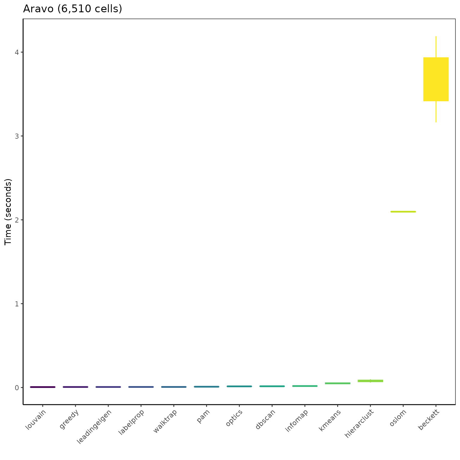

ggplot(mbm_plot[which(mbm_plot$dataset == "Fish (65910 cells)"), ],
       aes(reorder(algorithm, time_sec), time_sec)) +
  geom_boxplot(aes(color = reorder(algorithm, time_sec),
                   fill = reorder(algorithm, time_sec)), show.legend = FALSE) +
  scale_color_viridis_d("Algorithm") +
  scale_fill_viridis_d("Algorithm") +
  labs(title = "European fish (65,910 cells)",
       x = "", y = "Time (seconds)") +
  theme_classic() +
  theme(panel.border = element_rect(fill = NA),
        axis.text.x = element_text(angle = 45, vjust = 1, hjust = 1))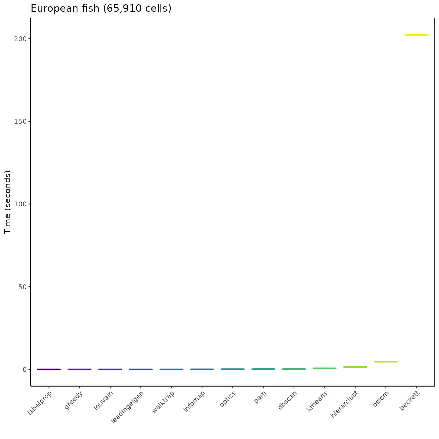

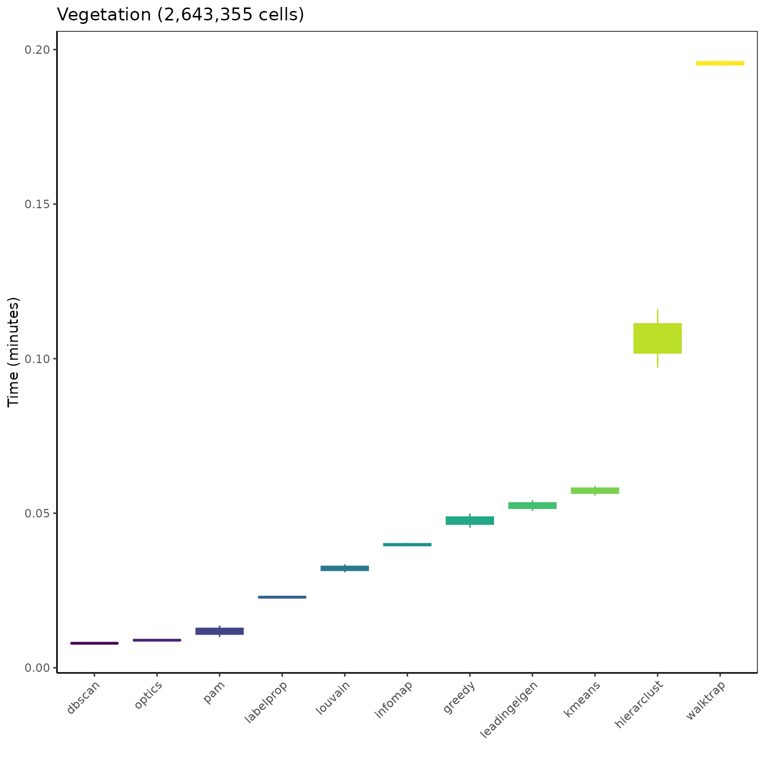
OSLOM and Beckett too slow, not ran so far on the Vegetation data.

ggplot(mbm_plot[which(mbm_plot$dataset == "Vegetation (2643355 cells)"), ],
       aes(reorder(algorithm, time_min), time_min)) +
  geom_boxplot(aes(color = reorder(algorithm, time_min),
                   fill = reorder(algorithm, time_min)), show.legend = FALSE) +
  scale_color_viridis_d("Algorithm") +
  scale_fill_viridis_d("Algorithm") +
  labs(title = "Vegetation (2,643,355 cells)", x = "", y = "Time (minutes)") +
  theme_classic() +
  theme(panel.border = element_rect(fill = NA),
        axis.text.x = element_text(angle = 45, vjust = 1, hjust = 1))

Pierre Denelle, Boris Leroy and Maxime Lenormand

2024-04-19

1. Datasets

1.1. Vegemat

1.2. European fish

1.3. Aravo

2. Microbenchmark